3.2.2. 窗函数及其性质
概念
实例
窗函数比较
实验内容
产生 \(f=100Hz\) 的余弦信号 \(x(t)\) , 采样率为 \(F_s = 1000Hz\) , 采样时间 \(T_s = 0.5s\) , 对信号 \(x(t)\) 施加六种窗函数, 窗函数持续时间 \(T_w = T_s = 0.5s\) , 并对加窗前后的数据进行快速傅里叶变换.
hammingcosineblackmangaussian, \({\rm{std}} = 100\)tukey, \(α= 10\)kaiser, \(β= 10\)
实验代码
1 2 3 4 5 6 7 8 9 10 11 12 13 14 15 16 17 18 19 20 21 22 23 24 25 26 27 28 29 30 31 32 33 34 35 36 37 38 39 40 41 42 43 44 45 46 47 48 49 50 51 52 53 54 55 56 57 58 59 60 61 62 63 64 65 66 67 68 69 70 71 72 73 74 75 | import numpy as np
from scipy import signal
import matplotlib.pyplot as plt
f = 100
Fs = 1000
T = 0.5
Tw = 0.5
Ns = int(T * Fs)
Nw = int(Tw * Fs)
t = np.linspace(0, T, Ns)
tw = np.linspace(0, Tw, Nw)
x = np.cos(2 * np.pi * f * t)
# windn = ('tukey', 10)
# windn = ('kaiser', 10)
# windn = ('gaussian', 100)
# windn = ('hamming')
# windn = ('cosine')
windn = ('blackman')
window = signal.get_window(windn, Nw)
print(Nw, len(window))
xfft = np.fft.fft(x)
ffft = np.fft.fftfreq(x.shape[-1])
idx = 0
y = x.copy()
y[idx:idx + Nw] = x[idx:idx + Nw] * window
print(y.shape, t.shape)
plt.figure(figsize=(10, 10))
plt.subplot(221)
plt.grid()
plt.plot(t, x)
plt.title('signal')
plt.xlabel('Time/s')
plt.ylabel('Amplitude')
plt.subplot(222)
plt.grid()
plt.plot(tw, window)
plt.title('window: ' + str(windn))
plt.xlabel('Time/s')
plt.ylabel('Amplitude')
plt.subplot(223)
plt.grid()
plt.plot(t, y)
plt.title('applied window on signal')
plt.xlabel('Time/s')
plt.ylabel('Amplitude')
yfft = np.fft.fft(y)
plt.subplot(224)
plt.grid()
plt.plot(ffft * Fs, np.abs(xfft), '-b')
plt.plot(ffft * Fs, np.abs(yfft), '-r')
plt.title('FFT of signal')
plt.legend(['orignal', 'windowed'])
plt.xlabel('Frequency/Hz')
plt.ylabel('Amplitude')
plt.show()
|
实验结果

图 3.1 effect of hamming window function
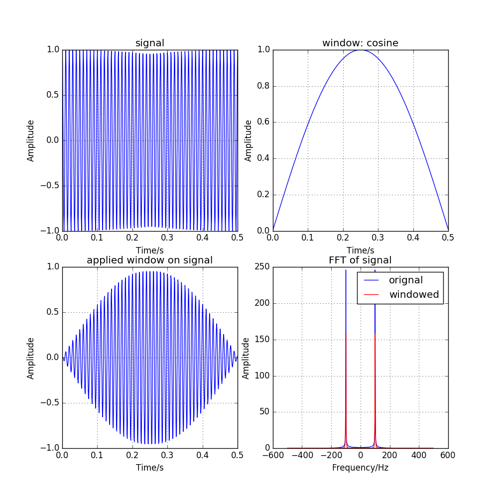
图 3.2 effect of cosine window function
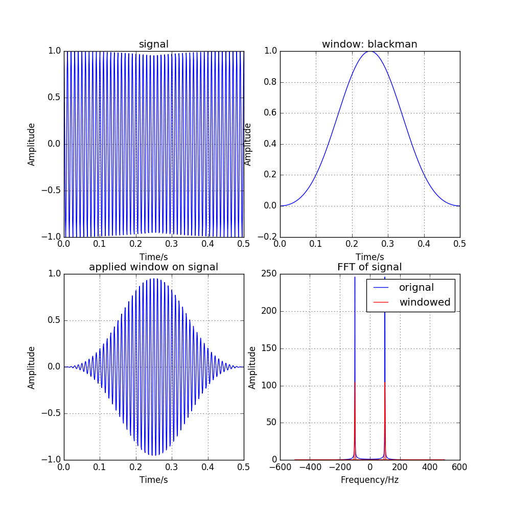
图 3.3 effect of blackman window function

图 3.4 effect of gauss window function, with \({\rm{std}} = 100\)
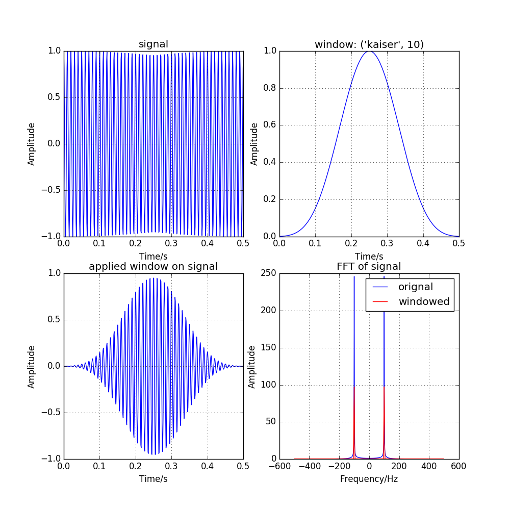
图 3.5 effect of kaiser window function, with \({\beta} = 10\)
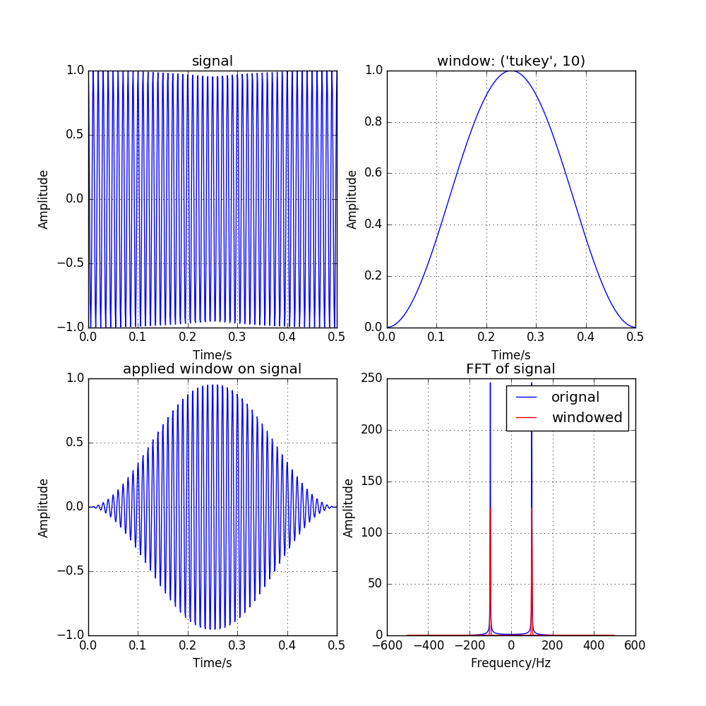
图 3.6 effect of tukey window function, with \({\alpha} = 10\)