1.1. 线性调频信号
1.1.1. 线性调频信号
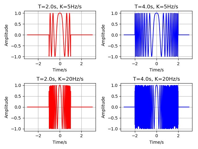
线性频率调制信号 (Linear Frequency Modulated , LFM) 简称 线性调频信号 (Chirp) , 之所以称之为 线性调频 是因为其频率随时间呈线性变化, 数学表示为:
其中, \(t\) 为时间, 单位为 \(\text s\) , \(K\) 为线性调频率, 可正可负, 单位为 \(\text{Hz/s}\), \(T\) 为脉冲宽度, 单位为 \(s\), 在脉冲持续时间内, 频率调制带宽为 \(B=|K|T\), 时间带宽积(Time Bandwidth Product, TBP)为 \({\rm TBP}=BT=|K|T^2\), \({\rm rect}\left(\frac{t}{T}\right)\) 为矩形窗函数, 只是对信号加了一定大小的窗, 窗大小由 \(T\) 决定,
提示
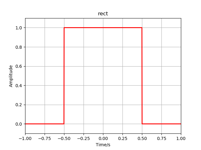
矩形窗函数的表达式如下:
脉冲相位 \(\phi(t) = \pi Kt^2\) 对时间取微分得到
即频率随时间线性变化, 因而称之为线性调频信号. 实际系统中, 可能会有一个初始相位 \(\phi_0\), 并且通常会把该信号加载到一个较高频率的载波 \({\rm exp}\left\{2j\pi F_c t\right\}\) 上发射, 从而有最终的发射信号为
1.1.2. 线性调频信号的频谱
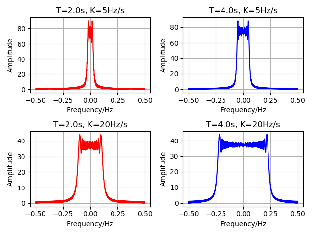
线性调频信号 \(s(t)={\rm rect}\left(\frac{t}{T}\right){\rm exp}\{j\phi(t)\}\) 的频谱为
很难直接求解出 式.1.17 所示积分解, 线性调频信号的性质, 决定了可以利用驻定相位原理 (Principle of Stationary Phase, PoSP) [1] 求解该积分的近似解. 在PoSP中, 将信号相位对于时间的导数为零的点称为驻留点, 在该点附近, 信号的相位是缓变的, 其值对积分的贡献大, 而在该区域之外的两侧, 是捷变的, 其正负部分几乎相互抵消, 积分为零, 因而, 积分值主要取决于驻留点附近的缓变区域. 只要时间带宽积 \({\rm TBP}\) 足够大, 利用POSP原理求得的积分解就是十分准确的.
提示
PoSP原理表明, 对于一个包络为 \(w(t)\) (时间缓变), 调制相位为 \(\phi(t)\) (时间捷变)的线性或近似线性调频信号 \(g(t)=w(t){\rm exp}\{j\phi(t)\}\), 其频谱可以近似为
其中, \(C=\sqrt{2\pi /|\phi''(t_s)|}\) 为一常数, \(w\left(t(f)\right)\) 为频域包络, \(\theta\left(t(f)\right)\) 为频域相位, \(\theta(t)=\phi(t)-2\pi ft\) 为时域相位, \(t(f)\) 由时频关系确定, \(\frac{\pi}{4}\) 前的符号与 \(\phi''(t_s)\) 的符号一致, \(t_s\) 为驻留点, \(C, \frac{\pi}{4}\) 通常可以被忽略. 线性调频信号的详细推导见 https://www.cnblogs.com/archerC/p/9359289.html
对于不含载频和初始相位的信号, 被积相位为 \(\theta(t)=\phi(t) - 2\pi ft=\pi Kt^2 - 2\pi ft\), 令 \({\rm d}{\theta(t)}/{\rm d}t=0\), 求得 \(f=Kt, t=f/K\), 则驻留点为 \(t_s=f/K\), 从而有 \(C=\sqrt{2\pi /|2\pi K|}=\sqrt{1/|K|}\), \(w(t(f))={\rm rect}(f/K)\) \(\theta(t(f))=\phi(f/K) - 2\pi f^2/K=-\pi {f^2}/K\), 最终得到该信号的频谱
对于含载频和初始相位的信号, 被积相位为 \(\theta(t)=\phi(t) - 2\pi ft=\phi_0 + 2\pi F_c t + \pi Kt^2 - 2\pi ft\), 令 \({\rm d}{\theta(t)}/{\rm d}t=0\), 求得 \(f=F_c+Kt, t=(f-F_c)/K\), 则驻留点为 \(t_s=(f-F_c)/K\), 从而有 \(C=\sqrt{2\pi /|2\pi K|}=\sqrt{1/|K|}\), \(w(t(f))={\rm rect}((f-F_c)/K)\), \(\theta(t(f))=\phi((f-F_c)/K) - 2\pi f(f-F_c)/K=-\pi (f-F_c)^2/K\), 最终得到该信号的频谱
1.1.3. 实验仿真
生成分析LFM
实验代码
python 代码如下
import matplotlib.pyplot as plt
import numpy as np


def rect(x):
    r"""
    Rectangle function:
        rect(x) = {1, if |x|<= 0.5; 0, otherwise}
    """
    return np.where(np.abs(x) >= 0.5, 0, 1)


def chirp(t, T, Kr):
    """
    Create a chirp signal :
        S_{tx}(t) = rect(t/T) * exp(1j*pi*Kr*t^2)
    """
    return rect(t / T) * np.exp(1j * np.pi * Kr * t ** 2)


Ns = 1000
t = np.linspace(-1, 1, Ns)
yrect = rect(t)

plt.figure()
plt.plot(t, yrect, '-r', linewidth=2)
plt.axis([-1, 1, -0.1, 1.1])
plt.grid()
plt.xlabel('Time/s')
plt.ylabel('Amplitude')
plt.title('rect')
plt.show()

Kr1 = 5
Kr2 = 20
T1 = 2.0
T2 = 4.0
t = np.linspace(-3, 3, Ns)
ychirp1 = chirp(t, T1, Kr=Kr1)
ychirp2 = chirp(t, T2, Kr=Kr1)

ychirp3 = chirp(t, T1, Kr=Kr2)
ychirp4 = chirp(t, T2, Kr=Kr2)

plt.figure()
plt.subplot(221)
plt.grid()
plt.plot(t, ychirp1, '-r')
plt.xlabel('Time/s')
plt.ylabel('Amplitude')
plt.title("T=" + str(T1) + "s, K=" + str(Kr1) + "Hz/s")
plt.subplot(222)
plt.grid()
plt.plot(t, ychirp2, '-b')
plt.xlabel('Time/s')
plt.ylabel('Amplitude')
plt.title("T=" + str(T2) + "s, K=" + str(Kr1) + "Hz/s")
plt.subplot(223)
plt.grid()
plt.plot(t, ychirp3, '-r')
plt.xlabel('Time/s')
plt.ylabel('Amplitude')
plt.title("T=" + str(T1) + "s, K=" + str(Kr2) + "Hz/s")
plt.subplot(224)
plt.grid()
plt.plot(t, ychirp4, '-b')
plt.xlabel('Time/s')
plt.ylabel('Amplitude')
plt.title("T=" + str(T2) + "s, K=" + str(Kr2) + "Hz/s")
plt.tight_layout()
plt.show()

# ==================compute spectral

ychirp1_fft = np.fft.fft(ychirp1)
ychirp2_fft = np.fft.fft(ychirp2)
ychirp3_fft = np.fft.fft(ychirp3)
ychirp4_fft = np.fft.fft(ychirp4)

ychirp1_fft = np.fft.fftshift(ychirp1_fft)
ychirp2_fft = np.fft.fftshift(ychirp2_fft)
ychirp3_fft = np.fft.fftshift(ychirp3_fft)
ychirp4_fft = np.fft.fftshift(ychirp4_fft)

f = np.fft.fftfreq(t.shape[-1])
# print(f)
f = np.fft.fftshift(f)
# print(f)

plt.figure()
plt.subplot(221)
plt.grid()
plt.plot(f, np.abs(ychirp1_fft), '-r')
plt.xlabel('Frequency/Hz')
plt.ylabel('Amplitude')
plt.title("T=" + str(T1) + "s, K=" + str(Kr1) + "Hz/s")
plt.subplot(222)
plt.grid()
plt.plot(f, np.abs(ychirp2_fft), '-b')
plt.xlabel('Frequency/Hz')
plt.ylabel('Amplitude')
plt.title("T=" + str(T2) + "s, K=" + str(Kr2) + "Hz/s")
plt.subplot(223)
plt.grid()
plt.plot(f, np.abs(ychirp3_fft), '-r')
plt.xlabel('Frequency/Hz')
plt.ylabel('Amplitude')
plt.title("T=" + str(T1) + "s, K=" + str(Kr1) + "Hz/s")
plt.subplot(224)
plt.grid()
plt.plot(f, np.abs(ychirp4_fft), '-b')
plt.xlabel('Frequency/Hz')
plt.ylabel('Amplitude')
plt.title("T=" + str(T2) + "s, K=" + str(Kr2) + "Hz/s")
plt.tight_layout()
plt.show()