2.1. 监督学习实践1 - 回归与优化
源自 UFLDL Tutorial , 原始代码可以从这里( GitHub repository )一次性下载. 需要注意的是有些数据需要自己去下载, 比如, 在做PCA的练习时, 需要下载MNIST数据集, 可以到 THE MNIST DATABASE 下载.
2.1.1. 线性回归
线性回归预测房价
Exercise 1A:线性回归预测房价, 只需补充目标函数及其梯度, 计算公式见原网页 :
补充代码
linear_regression.m
%%% YOUR CODE HERE %%%
theta = theta';
%Compute the linear regression objective
for j = 1:m
    f = f + (theta*X(:,j) - y(j))^2;
end
f = f/2;

%Compute the gradient of the objective
for j = 1:m
    g = g + X(:,j)*(theta*X(:,j) - y(j));
end
实验结果
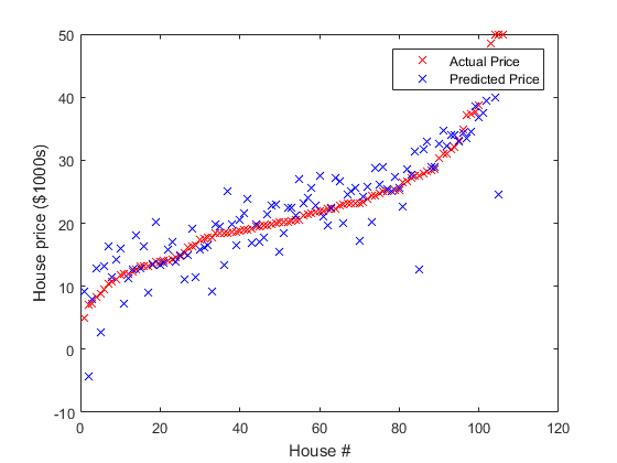
如原文所述, 训练和测试误差一般在\(4.5\)和\(5\)之间, 本人实验结果如 图 2.17 所示:
Optimization took 1.780584 seconds.
RMS training error: 4.731236
RMS testing error: 4.584099
2.1.2. Logistic Regression
上面的线性回归有两个特点:
预测连续值(房价);
输出是输入的 线性函数( \(y=h_{\theta}(x)=\theta^Tx\) );
代价函数为均方误差函数.
Logistic Regression:
预测离散值, 通常用于分类;
输出是输入的非线性函数(sigmoid或Logistic):\(y=h_{\theta}(x)=\sigma(\theta^Tx)\), \(\sigma(z)={1\over 1+exp(-z)}\) ;
代价函数取交叉熵(概率模型推), 最大似然, 见CS229 Notes).
Logistic Regression手写体分类
Logistic分类, 用于手写体. 只需补充目标函数及其梯度, 计算公式见原网页, 推导见 CS229 Notes :
补充代码 与线性回归基本相同, 只是假设\(y=h_{\theta}(x)=\sigma(\theta^Tx)\), \(\sigma(z)={1\over 1+exp(-z)}\)为sigmoid函数, 不再是线性函数.
%%% YOUR CODE HERE %%%

%Compute the linear regression objective and it's gradient
for j = 1:m
    coItem = sigmoid(theta'*X(:,j));
    f = f - y(j)*log(coItem) - (1-y(j))*log(1-coItem);
    g = g + X(:,j)*(coItem-y(j));
end
实验结果
如原网页所述, 最终训练和测试精度都为100%, 本人实验结果:
Optimization took 15.115248 seconds.
Training accuracy: 100.0%
Test accuracy: 100.0%
2.1.3. Vectorization
补充代码
需要取消ex1a_linreg.m和ex1b_logreg.m文件中下面的注释:
ex1a_linreg.m
% theta = rand(n,1);
% tic;
% theta = minFunc(@linear_regression_vec, theta, options, train.X, train.y);
% fprintf('Optimization took %f seconds.\n', toc);
ex1b_logreg.m
% theta = rand(n,1)*0.001;
% tic;
% theta=minFunc(@logistic_regression_vec, theta, options, train.X, train.y);
% fprintf('Optimization took %f seconds.\n', toc);
linear_regression_vec.m
%%% YOUR CODE HERE %%%
f = (norm(theta'*X - y))^2 / 2;
g = X*(theta'*X-y)';
logistic_regression_vec.m
%%% YOUR CODE HERE %%%
coItem = sigmoid(theta'*X);
f = -log(coItem)*y' -log(1-coItem)*(1-y)';
g = X*(coItem-y)';
实验结果
速度快了好些, 如下:
线性回归:
Optimization took 0.032485 seconds.(矢量化前约0.3s)
RMS training error: 4.023758
RMS testing error: 6.783703
Logistic分类:
Optimization took 3.419164 seconds.(矢量化前约12s)
Training accuracy: 100.0%
Test accuracy: 100.0%
2.1.4. Debugging: Gradient Checking
补充代码 下面是一次进行上述线性回归Logistic分类练习的梯度检验代码
grad_check_demo.m
%% for linear regression

% Load housing data from file.
data = load('housing.data');
data=data'; % put examples in columns

% Include a row of 1s as an additional intercept feature.
data = [ ones(1,size(data,2)); data ];

% Shuffle examples.
data = data(:, randperm(size(data,2)));

% Split into train and test sets
% The last row of 'data' is the median home price.
train.X = data(1:end-1,1:400);
train.y = data(end,1:400);

test.X = data(1:end-1,401:end);
test.y = data(end,401:end);

m=size(train.X,2);
n=size(train.X,1);

% Initialize the coefficient vector theta to random values.
theta0 = rand(n,1);

num_checks = 20;
% without vectorize
average_error = grad_check(@linear_regression, theta0, num_checks, train.X, train.y)
% vectorize
average_error = grad_check(@linear_regression_vec, theta0, num_checks, train.X, train.y)

%% for Logistic Classification
binary_digits = true;
[train,test] = ex1_load_mnist(binary_digits);

% Add row of 1s to the dataset to act as an intercept term.
train.X = [ones(1,size(train.X,2)); train.X];
test.X = [ones(1,size(test.X,2)); test.X];

% Training set dimensions
m=size(train.X,2);
n=size(train.X,1);

% Train logistic regression classifier using minFunc
options = struct('MaxIter', 100);

% First, we initialize theta to some small random values.
theta0 = rand(n,1)*0.001;

num_checks = 20;
% without vectorize
average_error = grad_check(@logistic_regression, theta0, num_checks, train.X, train.y)
% vectorize
average_error = grad_check(@logistic_regression_vec, theta0, num_checks, train.X, train.y)
实验结果
验证20次的平均误差分别为:
1.7030e-05(linear)
1.2627e-05(linear_vec)
6.0687e-06(Logistic)
8.1527e-06(Logistic_vec)