1.2. 凸多边形区域填充
1.2.1. 问题分析
1.2.2. 填充算法
扫描线法
夹角和法
内部点与各顶点夹角和为360度.
多边形方程法
该方法的核心思想是 多边形内的点满足多边形区域的边构成的不等式方程组, 设有由 \(N\) 个有序顶点 \({\mathbb P}=\{(x_i, y_i)^T\}_{i=1}^N\) 按顺序(逆时针或顺时针)构成的多边形区域 \(\mathcal P\).
若按逆时针方向, 则多边形内的区域可以表示为不等式方程组
若按顺时针方向, 则多边形内的区域可以表示为不等式方程组
其中, \(a_n = y_n-y_{n+1}\), \(b_n = x_{n+1}-x_{n}\), \(c_{n} = y_{n+1}(x_{n}-x_{n+1})-x_{n+1}(y_{n}-y_{n+1})\), \(n=1,2,\cdots, N\), 且 \(x_{N+1} = x_{1}, y_{N+1} = y_{1}\).
综上可知, 凸多边形区域内的点对应的凸多边形不等式方程组中的不等式同号.
故若要判断一点 \(P_0=(x_0, y_0)^T\) 是否在某凸多边形区域内, 只需要将改点坐标代入 式.1.11, 判断是否同号即可. 若满足则待填充点在多边形区域内, 反之不在.
1.2.3. 实验与分析
实验1
实验设置
假如对由有序顶点集合 \(\{(0, 0), (200, 0), (200, 100), (0, 100)\}\) 确定的方形区域 \(\mathcal R\) 内的凸多边形区域 \(\mathcal P\) 进行区域填充, 其中, \(\mathcal P\) 由有序顶点集合 \(\{(50, 50), (40, 40), (42, 25)\), \((55, 5), (65, 20), (70, 40), (60, 50)\}\) 确定. 记水平与垂直方向上的离散化尺度分别为 \(d_x, d_y\), 分析对比不同尺度下, 各种凸多边形填充算法的执行效率与填充效果.
实验代码
实验中用到的代码可在 这里 和 这里 下载, 主程序代码见 代码 1.6
1 2 3 4 5 6 7 8 9 10 11 12 13 14 15 16 17 18 19 20 21 22 23 24 25 26 27 28 29 30 31 32 33 34 35 36 37 38 39 | clear all
close all
clc
H = 100;
W = 200;
% dy = 0.1;
% dx = 0.1;
% dy = 0.5;
% dx = 0.5;
dy = 1;
dx = 1;
Polygon = [50 50; 40 40; 42 25; 55 5; 65 20; 70 40; 60 50]; % Anti Clockwise
% Polygon = [60 50; 70 40; 65 20; 55 5; 42 25; 40 40; 50 50]; % Clockwise
% Polygon = [50 50; 40 40; 55 5; 70 40; 58 42];
[y, x] = meshgrid(1:dy:H, 1:dx:W);
y = y(:);
x = x(:);
Points = [x y];
tic;
s1 = isincvxplg(Points, Polygon, 'Angle');
toc;
tic;
s2 = isincvxplg(Points, Polygon, 'PolygonEquations');
toc;
figure
hold on
subplot(121)
cpplot(Polygon, '-r', 'linewidth', 2)
opplot(Points(s1, :), '*r', 'linewidth', 1)
subplot(122)
cpplot(Polygon, '-r', 'linewidth', 2)
opplot(Points(s2, :), '*r', 'linewidth', 1)
|
凸多边形区域填充算法核心代码如 代码 1.7 所示:
1 2 3 4 5 6 7 8 9 10 11 12 13 14 15 16 17 18 19 20 21 22 23 24 25 26 27 28 29 30 31 32 33 34 35 36 37 38 39 40 41 42 43 44 45 46 47 48 49 50 51 52 53 54 55 56 57 58 59 60 61 62 63 64 65 66 67 68 69 70 71 72 73 74 75 76 77 78 79 | function [ s ] = isincvxplg( Points, Polygon, Method )
%ISINCVXPLG judges whether a point is in a convex polygon area
%
% s = ISINCVXPLG( Points, Polygon ) returns the the status (in Polygon --> 1,
% not in Polygon --> 0) of each point in Points.
%
% s = ISINCVXPLG( Points, Polygon, Method ) returns the the status (in Polygon --> 1,
% not in Polygon --> 0) of each point in Points using method 'Method'.
% Points: N-2 array, [x y;x y;...]
% Polygon: L-2 array, [x y;x y;...]
% Method: 'Angle' (default), 'PolygonEquations'
%
% Examples
% --------
%
% Points = [1 1; 2 2;3 3];
% Polygon = [1 2;1.5 1;2.5 1;3 2;2 3];
% cpplot(Polygon, '-r', 'linewidth', 2)
% hold on
% opplot(Points, '*r', 'linewidth', 1)
% s = isinpolygon(Points, Polygon)
% s =
%
% 0
% 1
% 0
% s = isinpolygon(Points, Polygon, 'PolygonEquations')
%
%
% See also isincircle.
%
% Copyright 2019-2030 Zhi Liu, https://iridescent.ink/.
%
if nargin < 3
Method = 'Angle';
end
EPS = 1e-6;
nPoints = size(Points, 1);
nVertex = size(Polygon, 1);
PI2 = pi + pi;
Polygon = Polygon(:, 1:2);
s = false(nPoints, 1);
if strcmp(Method, 'Angle')
for n = 1:nPoints
Pg = bsxfun(@minus, Polygon, Points(n, :));
Pa = Pg(1:nVertex, :);
Pb = [Pg(2:nVertex, :); Pg(1, :)];
A = angle2(Pa, Pb, 0);
A = abs(A);
sumA = sum(A, 1);
if abs(sumA - PI2) < EPS
s(n) = 1;
else
s(n) = 0;
end
end
end
if strcmp(Method, 'PolygonEquations')
Q = mean(Polygon, 1);
Ls = zeros(nVertex, 4); % edges
for nv = 1:nVertex-1
Ls(nv, :) = [Polygon(nv, :), Polygon(nv+1, :)];
end
Ls(end, :) = [Polygon(end, :), Polygon(1, :)];
A = Ls(:, 2) - Ls(:, 4);
B = Ls(:, 3) - Ls(:, 1);
C = Ls(:, 4) .* (Ls(:, 1) - Ls(:, 3)) - Ls(:, 3) .* (Ls(:, 2) - Ls(:, 4));
for n = 1:nPoints
fp = A * Points(n, 1) + B * Points(n, 2) + C;
s(n) = (sum((fp >= 0))== nVertex) || (sum((fp > 0)) == 0);
end
end
end
|
实验结果
我们在MatlabR2019上实现上述算法, 硬件平台为Intel® Xeon(R) CPU E5-2696 v3 @ 2.30GHz × 36, 实验中仅使用单线程, 运行时间如 表 1.1 所示, 填充效果如 图 1.12 所示. 对比表格与填充效果图可知, 多边形方程法计算复杂度更低, 耗时极短, 效率更高.
方法 |
\(d_x=d_y=1\) |
\(d_x=d_y=0.5\) |
\(d_x=d_y=0.1\) |
|---|---|---|---|
夹角和法 |
0.758408s |
2.397315s |
57.775898s |
多边形方程法 |
0.020063s |
0.056518s |
0.943451s |
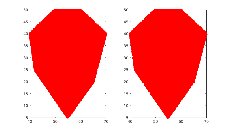
图 1.12 凸多边形区域填充结果对比图. 夹角和法(左), 多边形方程法(右)